Join Copernicus Climate Data Store Data with Socio-Economic and Opinion Poll Data

In this series of blogposts we will show how to collect environmental data from the EU’s Copernicus Climate Data Store, and bring it to a data format that you can join with Eurostat’s socio-economic and environmental data. We have shown in a previous blogpost how to connect this to survey (opinion poll) and tax data, and a real policy problem in Belgium. We will create now subsequent tutorials to do more!

But first, why are we doing this? The European Union and its members states are releasing every year more and more data for open re-use since 2003, yet these are often not used in the EU’s data dissemination projects (the observatories) or in EU-funded research. We believe that there are many reasons behind this. Whilst more and more people can conduct business, scientific or policy analysis programmatically or with statistical software, knowledge how to systematically collect the data from the exponentially growing availability is not everybody’s specialty. And the lack of documentation, and high re-processing and validation need for open data is another drawback.

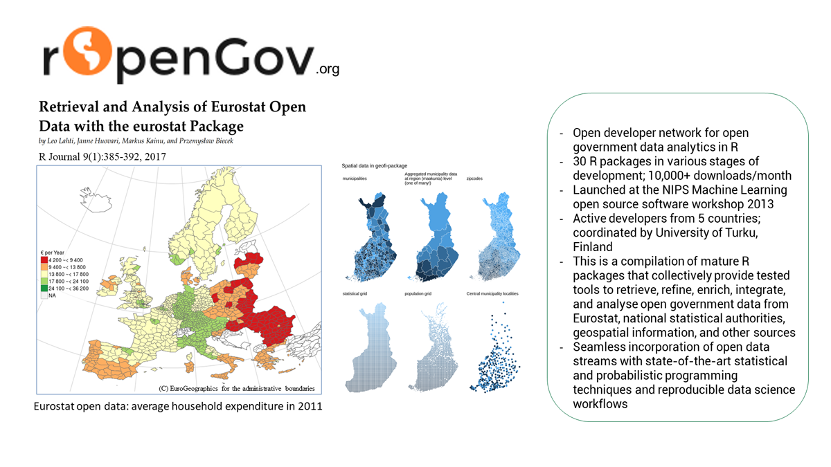
rOpenGov has long been producing high-quality, peer-reviewed R packages to work with open data, but their use is not for all. In an open collaboration, where you can join, too, rOpenGov teamed up with open source developers, knowledgeable data curators, and a service developer team lead by the Dutch reproducible research start-up Reprex to create a sustainable infrastructure that is permanently collecting, processing, documenting and visualizing open data. What we do is that we access open data (that is not always available for direct download) and re-process it to usable data that is tidy to be integrated with your existing data or databases. We are competing for the EU Datathon Challenge 1: supporting a European Green Deal agenda with open data as a service, and research as a servcie, and you are more than welcome to join our effort as a developer, a data curator, or as an occasional contributor to open government packages.

Register to the Copernicus Climate Data Store

Koen Hufkens, Reto Stauffer and Elio Campitelli created the ecmwfr R package for programmatically accessing the Copernicus Data Store service. Follow the CDS Functionality vignette to get started.

You will need to create a Register yourself for CDS services after accepting the Terms and conditions.

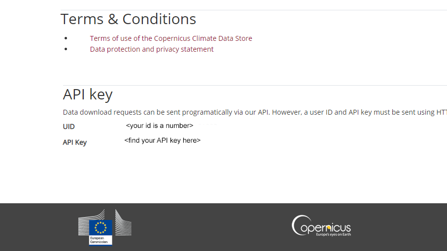
wf_set_key(user = "12345", 
           key = "00000000-aaaa-b1b1-0000-a1a1a1a1a1a1", 
           service = "cds")

You can check if you were successful with:

ecmwfr::wf_get_key(user = "12345", service = "cds")

Get the Data

Let us formulate our first request:

request_lai_hv_2019_06 <- list(
  "dataset_short_name" = "reanalysis-era5-land-monthly-means",
  "product_type"   = "monthly_averaged_reanalysis",
  "variable"       = "leaf_area_index_high_vegetation",
  "year"           = "2019",
  "month"          =  "06",
  "time"           = "00:00",
  "area"           = "70/-20/30/60",
  "format"         = "netcdf",
  "target"         = "demo_file.nc")

lai_hv_2019_06.nc  <- wf_request(user = "<your_ID>",
                     request = request_lai_hv_2019_06 ,
                     transfer = TRUE,
                     path = "data-raw",
                     verbose = FALSE)

Effective Leaf Area Index

You can find this data either in global computer raster images, or in re-processed monthly averages. Working with the raw data is not very practical – in case of cloudy weather you have missing data, and the files are extremely huge for a personal computer. For the purposes of our Green Deal Data Observatory the monthly average values are far more practical, which are called monthly_averaged_reanalysis product types.

For compatibility with other R packages, convert the data with the from raster package from rSpatial.org.

lai_file <- here::here( "data-raw", "demo_file.nc")
lai_raster <- raster::raster(lai_file)

## Loading required namespace: ncdf4

Let us convert this to a SpatialDataPointsDataFrame class, which is an augmented data frame class with coordinates.

LAI_df <- raster::rasterToPoints(lai_raster, fun=NULL, spatial=TRUE)

Get The Map

With the help fo rOpenGov, we are creating various R packages to programmatically access open data and put them into the right format. The popular eurostat package is not only useful to download data from Eurostat, but also to map it.

In this case, we want to create regional maps. Europe has five levels of geographical regions: NUTS0 for countries, NUTS1 for larger areas like states, provinces; NUTS2 for smaller areas like countries, NUTS3 for even smaller areas. The LAU level contains settlemens and their surrounding areas.

Country borders change sometimes (think about the unification of Germany, or the breakup of Czechoslovakia and Yugoslavia), but they are relatively stable entities. Sub-national regional border change very-very frequently – since 2000 there were many thousand changes in Europe. This means that you must choose one regional boundary definition. The latest edition is NUTS2021 but most of the data available is still in the NUTS2016 format, and often you will find NUTS2013 or even NUTS2010 data around. Our Green Deal Data Observatory uses the NUTS2016 definition, because it is far the most used in 2021. An offspring of the eurostat package, regions helps you take care of NUTS changes when you work, and can convert your data to NUTS2021 if you later need it.

## sf at resolution 1:60 read from local file

## Warning in eurostat::get_eurostat_geospatial(resolution = "60", nuts_level =
## "2", : Default of 'make_valid' for 'output_class="sf"' will be changed in the
## future (see function details).

plot(map_nuts_2)

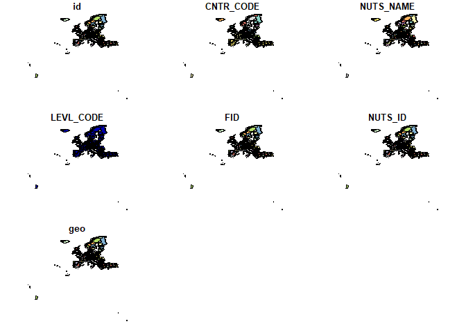
Our measurement of the average Effective Leaf Area Index is a raster data, it is given for many points of Europe’s map. What we need to do is to overlay this raster information of the statistical map of Europe. We use the excellent sp: R Classes and Methods for Spatial Data package for this purpose. The sp::over() function decides if a point of Leaf Area Index measurement falls into the polygon (shape) of a particular NUTS2 regions, for example, Zuid-Holland or South Holland in the Netherlands, or Saarland in Germany, or not. Then it averages with the mean() function those measurements falling in the area.

LAI_nuts_2 = sp::over(sp::geometry(
  as(map_nuts_2, 'Spatial')), 
  LAI_df,
  fn=mean)

Let’s call the average LAI index lai, and bind it to the Eurostat map:

names(LAI_nuts_2)[1] <- "lai"
LAI_sfdf <- bind_cols ( map_nuts_2, LAI_nuts_2 )

If you want to work with the data in a numeric context, you do not need the geographical information, and you can “downgrade” the SpatialDataPointsDataFrame to a simple data frame.

set.seed(2019) #to always see the same sample
LAI_sfdf %>%
  as.data.frame() %>%
  select ( all_of(c("NUTS_NAME", "NUTS_ID", "lai")) ) %>%
  sample_n(10)

##                      NUTS_NAME NUTS_ID lai
## 281                       Vest    RO42  NA
## 125                     Kassel    DE73  NA
## 69              Friesland (NL)    NL12  NA
## 237 Agri, Kars, Igdir, Ardahan    TRA2  NA
## 273                East Anglia    UKH1  NA
## 119                Prov. Liège    BE33  NA
## 61                   Bourgogne    FRC1  NA
## 275                      Essex    UKH3  NA
## 282                   Istanbul    TR10  NA
## 174                    Leipzig    DED5  NA

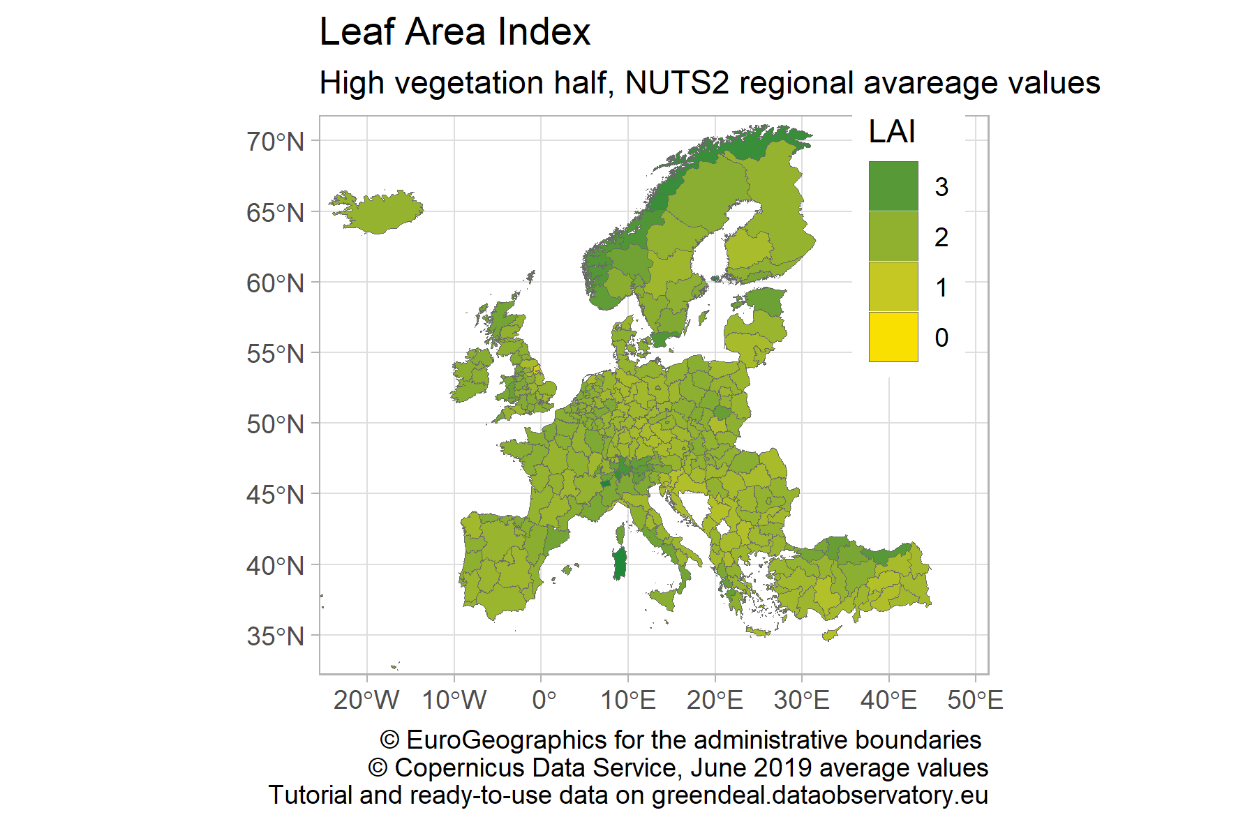
We’ll plot the map with ggplot2.

library(ggplot2)
library(sf)
ggplot(data=LAI_sfdf) + 
  geom_sf(aes(fill=lai),
          color="dim grey", size=.1) + 
  scale_fill_gradient( low ="#FAE000", high = "#00843A") +
  guides(fill = guide_legend(reverse=T, title = "LAI")) +
  labs(title="Leaf Area Index",
       subtitle = "High vegetation half, NUTS2 regional avareage values",
       caption="\ua9 EuroGeographics for the administrative boundaries 
                \ua9 Copernicus Data Service, June 2019 average values
                Tutorial and ready-to-use data on greendeal.dataobservatory.eu") +
  theme_light() + theme(legend.position=c(.88,.78)) +
  coord_sf(xlim=c(-22,48), ylim=c(34,70))

Data Integrity

Our Green Deal Data Observatory has a data API where we place the new data with metadata for programmatic download in CSV, JSON or even with SQL queries. For data integrity purposes, we are placing an authoritative copy on Zenodo (Green Deal Data Observatory Community). You can use this for scientific citations. We are also happy if you place your own climate policy related research data here, so that we can include it in our observatory. In our subsequent tutorials, we will show how to do this programmatically in R. This particular dataset (not only with the month June, which we selected to streamline the tutorial) is available here with the digital object identifier doi.org/10.5281/zenodo.4903940.

Join us

Join our open collaboration Green Deal Data Observatory team as a data curator, developer or business developer. More interested in antitrust, innovation policy or economic impact analysis? Try our Economy Data Observatory team! Or your interest lies more in data governance, trustworthy AI and other digital market problems? Check out our Digital Music Observatory team!