Regional Geocoding Harmonization Case Study - Regional Climate Change Awareness Datasets
Harmonizing sub-national geographical information
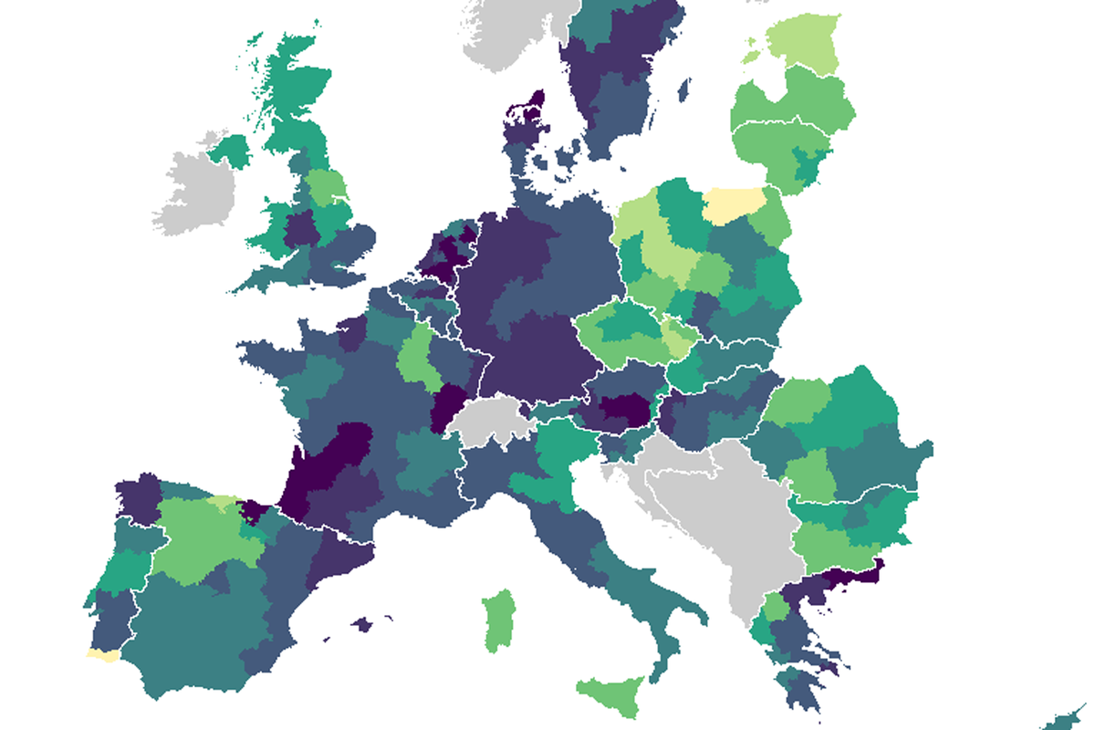 A better map after harmonization of geographical metadata.
library(regions)
library(lubridate)
library(dplyr)

if ( dir.exists('data-raw') ) {
  data_raw_dir <- "data-raw"
} else {
  data_raw_dir <- file.path("..", "..", "data-raw")
  }
Going beyond the national level
Let’s start with a dirty averaging by sub-national unit. The w1
weighting variable contains the post-stratification weight for the
national samples. The Eurobarometer samples represent nations (with the
exception of East and West Germany, Northern Ireland and Great Britain.)
The average of the w1 variable is 1.00 for each sample, but it is not
necessarily 1 for smaller territorial units. If sum(w)>1 for say,
AT23 it only means that the AT23 region was undersampled relatively
to the rest of Austria, and responses must be over-weighted in
post-stratification.
There is no way to make the samples become regionally representative, and a correct post-stratification would require further data about the sampel design. But we can simply adjust to over/undersampling by making sure that oversampled territorial averages are proportionally increased and undersampled ones are decreased. [Another ‘dirty’ averaging would be the use of an unweighted average, but our method is better, because it more-or-less adjusts gender and education level biases, but leaves intra-country regional biases in the sample.]
panel <- readRDS((file.path(data_raw_dir, "climate-panel.rds")))

climate_data <-  panel %>%
  mutate ( year = lubridate::year(date_of_interview)) %>%
  select ( all_of(c("isocntry", "geo", "w1")),
           contains("problem")
  )  %>%
  mutate (
    # use the post-stratification weights for national samples
    serious_world_problems_first = w1*serious_world_problems_first ,
    serious_world_problems_climate_change = w1*serious_world_problems_climate_change) %>%
  group_by (  .data$geo ) %>%
  summarise( serious_world_problems_first = mean(serious_world_problems_first, na.rm=TRUE),
             serious_world_problems_climate_change = mean (serious_world_problems_climate_change, na.rm=TRUE),
             mean_w1 = mean(w1)
             ) %>%
  mutate (
    # adjust for post-stratification weight bias due to regional over/undersampling
    climate_first = serious_world_problems_first / mean_w1,
    climate_mentioned = serious_world_problems_climate_change / mean_w1
    )
So, we averaged, weighted and adjusted the mentioning of climate change as the world’s most serious, or one of the most serious problems by NUTS regions.
Aggregation level
The problem is that most statistical data is available in for the NUTS
regional boundaries according to the NUTS2016 definition. However,
GESIS uses NUTS2013 regions, so 252 regional codes in the four survey
waves are invalid. Some data is available only on national level, but it
can be projected to regional level, because small countries like
Luxembourg have no regional divisions. Larger countries like Germany are
divided only on state level (NUTS1), while small countries are divided
on NUTS3 level.
This leads to various problems. Many data is available only on NUTS2
level, in which case NUTS1 data should be projected to its constituent
smaller NUTS2 regions, and NUTS3 level data must be aggregated up to
larger, containing NUTS2 levels.
Of course, we also must choose if we use `NUTS2013 or NUTS2016
boundaries. Sub-national boundaries have changed many thousand times in
the EU27 countries alone since 1999.
## # A tibble: 5 x 2
##   validate         n
##   <chr>        <int>
## 1 country         15
## 2 invalid        252
## 3 nuts_level_1   132
## 4 nuts_level_2   452
## 5 nuts_level_3   141
Recoding the Regions
Our regions package was designed to keep track of sub-national regional boundary changes. It can validate regional data codes, and to some extent carry out recoding, imputation or simple aggregation.
- Recoding means that the boundaries are unchanged, but the country changed the names/codes of regions, because there were other boundary changes which did not affect our observation unit.
- Imputation must not be done with usual, general imputation tools,
because our data is regionally structured. However, some imputations
are very simple, because we can use equality equasions like
MT=MT0,MT00. - Often the boundary change is additive, and merged territorial units can simple aggregated for comparison in earlier data.
regional_coding_2016 <- panel %>%
  mutate ( year = lubridate::year(date_of_interview)) %>%
  select (  all_of(c("isocntry", "geo", "region", "year") ) ) %>%
  distinct_all() %>%
  recode_nuts()

regional_coding_2013 <- panel %>%
  mutate ( year = lubridate::year(date_of_interview)) %>%
  select (  all_of(c("isocntry", "geo", "region", "year") ) ) %>%
  distinct_all() %>%
  recode_nuts( nuts_year = 2013)

climate_data_recoded <- climate_data %>%
  left_join ( regional_coding_2016, by = 'geo' ) %>%
  left_join ( regional_coding_2013 %>%
                select ( all_of(c("geo", "code_2013"))),
              by = "geo") %>%
  distinct_all()

saveRDS ( climate_data_recoded , file.path(tempdir(), "climate_panel_recoded_agr.rds"), version = 2)

# not evaluated
saveRDS( climate_data_recoded , file = file.path("data-raw", "climate_panel_recoded_agr.rds"))

Daniel Antal
Data Scientist & Founder of the Digital Music Observatory
My research interests include reproducible social science, economics and finance.